The Difference between Cumulative Distribution Function (CDF) and Probability Density Function (PDF)

Cumulative Distribution Function (CDF) vs Probability Distribution Function (PDF)

The Cumulative Distribution Function (CDF) of a random variable 'X' is the probability that the variable value is less than or equal to 'X'. It is the cumulative of all possible values between two defined ranges.On the other hand, Probability Distribution Function (PDF) is the probability of random variable 'X' equal to certain value. In other words it is a derivative of CDF.

Let us understand this with the example of Normal Distribution data. Normal Distribution curve is a bell shaped curve and is symmetric about its mean. its value extends from -ve infinity to +ve infinity. The curve extends indefinitely in both direction.

Consider a Normally Distributed Data with Mean = 494 and SD = 100. Let us calculate the  probability of random variable X between its mean and 500. Excel has NORMAL.DIST() function which returns CDF and PDF for a Normal Distribution. It takes four arguments namely; X, MEAN, SD and CUMULATIVE. The 4th argument CUMULATIVE is Boolean and if set to TRUE then the function returns CDF and if set to FALSE, the function returns PDF.

CDF = "NORM.DIST(500,494,100,TRUE)" = 0.5239 or  52.39%

PDF = "NORM.DIST(500,494,100,FALSE)" = 0.00 or  0%

In the above calculation CDF of 52.39% is a probability of X is from -infinity to 500. To get the probability of X between MEAN (494) and 500, subtract 50% from CDF, Hence the probability of X between MEAN and 500 is 2.39%.

Read More

The difference between DAYS and DAYS360 formulas

DAYS360:

The DAYS360 function is used  to calculate number of days between two dates. But it is based on the assumption that each month in a year has 30 days. This method is adopted in some financial institutions for the calculation of interest and other accounting purposes.

DAYS():
However Excel 2016 version has DAYS() formula which calculates the number of calendar days between two dates.

Read More

CAGR calculation in Excel

CAGR:

CAGR - Compounded Annual Growth Rate is a measure of growth over a period of time. It is usually calculated for number of years. Businesses use CAGR to measure the growth in their revenue over a period of time. In finance CAGR is used as a measure that indicates appreciation in the value of an Investment over a period of time.

Example:

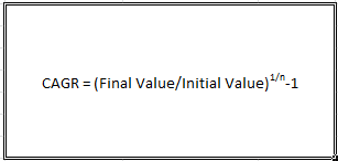
Suppose an initial investment of $10000 is made and its value appreciates to $17000 after 5 years. CAGR for this investment is calculated using the below formula.

                         

                                                          where n = no. of years

The CAGR for the above investment example is 0.11196 or 11.196%. Here, CAGR is equivalent to constant growth rate per year. (i.e. Constant growth of 11.196% for 5 consecutive years.

You can validate the CAGR by calculating Final Value using the initial value of $10000 and CAGR of 11.196%.

                                Final Value = $10000 * (1+0.11196)^5 = $17000

Read More

How to use SUMPRODUCT to calculate mean of Discreet Distribution

Discreet Distribution:

A Discreet Distribution is a distribution constructed from a random variable produced by non-negative whole numbers. MEAN or AVERAGE is nothing but Expected Value of a Discreet Distribution.

The MEAN of any discreet distribution is calculated by taking the sum of product of values and their probability of occurrence.In the below example, number of Diabetics out  of 5 people chosen randomly and probability of number of Diabetics in the sample.

MEAN of this discreet distribution is calculated using inbuilt function SUMPRODUCT as shown below. SUMPRODUCT takes two arguments, ARRAY1 and ARRAY2.
                               
                                                "=SUMPRODUCT(C2:C8,D2:D8)"

 The mean or the expected value of the above discreet distribution is 1.14.

Read More

How to convert number to words in Excel

In this example let us learn to build excel template to convert a three digit number to words. Consider a three digit number say 256 in cell B1. We need to get "Two Hundred and Fifty Six" in cell C1.

First create two separate table as shown below in sheet 2 of the workbook. Values have to be entered manually for the first time.

Now get 1st, 10th and 100th digits  in cells I1, I2 and I3 respectively using RIGHT function. Now divide each number by their digit of significance and take only integer portion of it using INT function. i.e.
                        J1 = INT(I1/H1) = 6
                        J2 = INT(I2/H2) = 5
                        J3 = INT(I3/H3) = 2

       

Now do a VLOOKUP of values in cell J1, J2 and J3 in Table1 and Table2 created in STEP1 shown in picture below.

Now, in cell L1 enter the formula "=CONCATENATE(K3,K2,K1)" to get the number in to words.

Now select cell C1 in  Sheet1 of the workbook and enter ="Sheet2!L1". Now  "Two Hundred and Fifty Six" appear in cell C1.

Read More

Stem and Leaf Diagram in Excel

Stem and Leaf Plots:

Stem and Leaf diagram is simple and useful tool to organize data into groups. Representing data in Stem and Leaf diagram gives the birds eye view of data and gives basic picture of how data is distributed across different Levels.

How to construct Stem and Leaf diagram?

Stem and Leaf plot is created by dividing the data set into two parts, a stem and a leaf. Stem is to the left side of the plot and consists most significant digit and number with less significance are leaves. For example,  number 78, 76, 71 will have 7 on stem and 8, 6, 1 are leaves. In case of 3 digit numbers two digits from left forms stem and 3rd forms leaves.

However the division of digits into stem and leaf is subjected to scope of study. Below is a sample stem and leaf diagram of marks secured by candidates in banking examination.

Below is a video demonstration of Stem and Leaf diagram simulator in Excel.

Read More

How to create barcode in Excel

This tutorial is aimed at generating barcode equivalent of a alphanumeric number into an Excel cell. There are different types of Barcodes, such as

EAN 13,
EAN 8,
UPC A,
UPC E,
Code 128,
 ITF 14 and
Code 39.

 The first step is to decide on the right Barcode type to create (or print) depending on requirement. In this tutorial, Code 128 standard is used for illustration. Once the barcode type is decided, download the TrueType font file from google. TrueType font file is similar to a notepad file with ".ttf" extension.

After downloading the file, copy the file to "C:\Windows\Fonts" of your windows installation directory. Now, open the file copied and click on Installation as shown in the picture.

Now, open new Excel workbook select any cell type any alpha numeric number and then change the font type to Code128 from the drop down of font style as shown below.

This will generate the barcode equivalent of a number.

Read More

How to use Goal Seek in Excel

Goal Seek is one of the most important tool in Excel which helps in calculating the value input when the output is known. In other words, it calculates the value of input for the desired value of output.

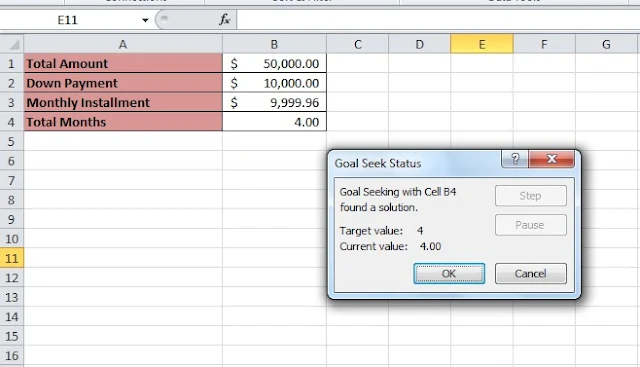
Consider an Example, where a product of $ 50000 is bought on installment basis. The down payment made at the time of purchase was $ 10000. The remaining balance of $ 40000 has to be paid in monthly installment of $ 5000 each. Now, let us calculate the the number of months, the installment to paid back.

In cell B4 enter the below formula to calculate the number  of months.

                                                 "=(B1-B2)/B3"

The number of months installment to be paid is 8.

Now, let us use goal seek to determine the change in monthly installment, if the buyer decides to pay installment in 4 months instead of 8.

1) Select Data > WhatIfAnalysis > Goal Seek>

2) Goal Seek pop up window has three fields namely set cell:, to value: and By changing Cell:

      set cell:
      set cell is always a cell that contains formula. In this example it is B4.

      to value:
      Enter 4 in to value field.
   
      by changing cell:
      As we are determining the value of monthly installment for which the the no. of months is 4,               enter B3 in this field and click OK.

3) Goal Seek determines the monthly installment value and populates the same as shown below.

     Note: Goal seek does not allow the changes to multiple cells simultaneously. Use solver AddIn to      set criteria for multiple cells (or multiple variables).                        

            

Read More

How to save an Excel Workbook as HTML document?!!

Saving an Excel workbook as HTML document is necessary whenever it is required to publish reports generated in Excel on Web portals. 

The following are the steps to save an Excel sheet as HTML document.

1) Open the Excel workbook which you want to save as HTML.

2) Select File menu and click "Save As" from drop down menu.

3) Now in "Save as" window pop up, type the name of the file and in "save as type" field select
    "save as single file web page".

4) Once the "save as type" is selected, check "selection :sheet" and click on publish as
shown below.

5) Now, In "publish as" pop up window, select the sheet which you want to publish as html document and change the name and path where you want to save document. Make sure that AutoRepublish checkbox is checked (to keep original file and HTML document synchronized) and click on Publish.

6) Now, the saved HTML page can be viewed in web browser. Changes made in the original file are        automatically reflected in web page on refreshing.

Read More

How to generate dummy data in Excel

Whenever you want to test a formula or build a data model involving complex business logic, It becomes necessary to create set of sample data by yourself to work with. RANDBETWEEN function is an useful tool to generate random numbers.

syntax:

RANDBETWEEN(lower value, upper value)


Consider a scenario where 10 three digit random numbers have to be generated.
Select cell B2 and type "=RANDBETWEEN(100, 999)"

Now, drag the formula upto cell B11 to get 10 thee digit random numbers.

Random numbers change every time you refresh the sheet or workbook.

Note: This function can be used to simulate random experiments, such as tossing of coin or rolling a die. For example, use "=RANDBETWEEN(1,6)" for rolling of a die.

Read More

How to use skip blanks feature in paste special option?!?

There exists a lot of confusion among excel users on usage of "skip blanks" feature in paste special. They expect the skip blanks to filter and paste the non blank cells but, skip blanks retains the original value of the destination cell if the corresponding cell in the source cell  is blank.

Let us understand this with an example. Consider two columns A and B with integers as shown below. The cell A4 in source column is left blank.

Now, copy the values in source column, i.e. from A2 to A7. 

Select cell B2 and right click and select paste special from context menu. Check 'values' and 'skip blanks' from paste special popup window and click OK. Now all the values in destination cell changes except for the cell B4 as shown in the picture below.

Read More

How to import file names of a folder into an Excel spreadsheet

Following are the steps to import list of file names from a folder in to an Excel sheet.

1) Select a folder in which the files to be imported are saved. In this case, I've selected AV files folder on my desktop with 4 files in it.

2) Now, hold the Shift key on keyboard and right click on the folder and then select "Open command window here" from the context menu as shown in the picture above.

3) Now the command window pops up with the present directory. Type "dir / b>filenames.xls" in the command prompt and hit Enter.

4) The new Excel workbook "filenames.xls" has been created in AV files folder with the list of file names in it as shown in the picture above.

Read More